Transport Block Size: The Fundamental Unit of Wireless Data Transmission
In the invisible symphony of wireless communication, where data flows as digital signals between your device and a cell tower, there exists a critical, yet often overlooked, maestro: the transport block. It is not merely a packet or a frame, but the fundamental, physical-layer unit of data that a network schedules, transmits, and acknowledges. Understanding transport block size is akin to understanding the blueprint of a data delivery system. It dictates efficiency, speed, and reliability. This concept sits at the very heart of how 4G LTE and 5G New Radio (NR) translate the theoretical promise of high-speed data into tangible bits received on your smartphone. For network engineers, it’s a daily tuning parameter. For performance optimization, it’s a key lever. And for anyone seeking a deep grasp of modern cellular technology, it’s an indispensable piece of the puzzle. This comprehensive guide will demystify transport block size, exploring its role, calculation, and profound impact on your wireless experience.
The Core Concept of a Transport Block
Imagine a freight train system where the train itself is the physical radio signal. The individual cargo containers loaded onto that train are the transport blocks. The network’s scheduler decides how many containers (transport blocks) to load onto each train (transmission time interval) based on the track quality (channel conditions) and the priority of the goods (QoS of the data). A transport block is therefore the basic data unit delivered from the higher layers (like the MAC layer) to the physical layer for actual transmission over the air.
It is more than just a lump of bits. Each transport block is wrapped with its own error-detecting CRC (Cyclic Redundancy Check), creating a self-contained package for reliability. The size of this package—the transport block size—is not fixed. It is dynamically determined for every single transmission, making it a cornerstone of the adaptive and efficient nature of modern cellular systems. This dynamic sizing is what allows your phone to download a large file rapidly in good coverage, yet maintain a stable connection for a voice call in a weak signal area.
Transport Blocks in the LTE Ecosystem
In the LTE architecture, the transport block is the payload carried by the shared data channel, the PDSCH (Physical Downlink Shared Channel) for downloads and the PUSCH (Physical Uplink Shared Channel) for uploads. The process is tightly orchestrated. The base station (eNodeB) continuously estimates the downlink channel quality for each user, primarily based on feedback reports like CQI (Channel Quality Indicator). Using this information, it selects a Modulation and Coding Scheme (MCS) and determines the available physical resources.
The combination of the selected MCS and the number of allocated resource blocks directly dictates the possible transport block size. LTE standards define a large but finite set of possible sizes, organized in lookup tables. The scheduler picks the index corresponding to the chosen MCS and resource allocation, which points to the precise block size to use. This ensures the block fits perfectly into the scheduled physical resources, maximizing spectral efficiency for that specific user at that exact moment.
The Evolution into 5G New Radio
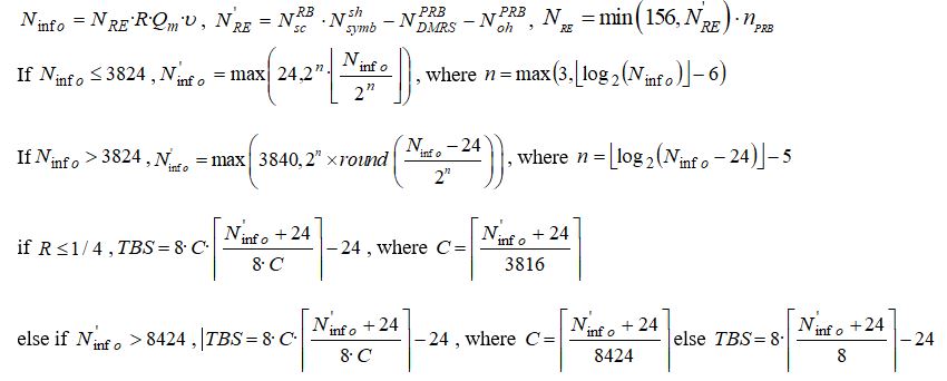
5G NR inherits the core concept of the transport block but introduces significant enhancements for greater flexibility and to support a wider range of use cases. While LTE’s transport block sizes were table-based, 5G employs a more formulaic approach, providing a finer granularity of possible sizes. This is crucial for supporting diverse services, from massive IoT (small, infrequent blocks) to enhanced mobile broadband (very large blocks) and ultra-reliable low-latency communications (optimized, time-critical blocks).
A key 5G innovation is the more explicit and dynamic link adaptation. The transport block size in 5G is a function of the allocated bandwidth, the symbol duration, the modulation order (QPSK, 16QAM, 64QAM, 256QAM, and now 1024QAM), and the target code rate. The gNodeB (5G base station) has more granular control, allowing it to tailor the block size with unprecedented precision to match the channel conditions and service requirements, pushing the boundaries of what is efficiently transmittable in a given scenario.
The Intricate Calculation Process
Calculating the transport block size is a multi-step procedure that bridges the gap between abstract channel quality and concrete physical resources. It begins with channel measurement. The user equipment (UE) measures the signal-to-interference-plus-noise ratio (SINR) and reports a channel quality indicator (CQI) back to the base station. This CQI is not a direct measure of speed but a recommendation for an MCS index that the UE believes it can decode with a reasonable block error rate (BLER), typically targeted at 10%.
The base station’s scheduler then interprets this CQI, considers other factors like buffer status and user priority, and finalizes an MCS. It also decides how many resource blocks (RBs) to allocate to the user. These two decisions—MCS and number of RBs—are the primary inputs. In LTE, these inputs are used to look up a TBS index in one table, which is then used with the number of RBs in a second, larger table to find the final transport block size. This table-driven approach ensures standardization but limits granularity.
Modulation, Coding, and Their Direct Impact
Modulation and coding are the twin engines that determine how densely information can be packed into a radio wave, and they have a direct, mathematical relationship with transport block size. Modulation (e.g., QPSK, 16QAM, 256QAM) defines how many bits can be carried per symbol. A higher order modulation like 256QAM carries 8 bits per symbol, while QPSK carries only 2. This directly scales the potential size of the data payload.
Coding adds redundancy for error correction. The code rate expresses the proportion of useful data bits to the total transmitted bits (data + redundancy). A high code rate (e.g., 0.9) means less redundancy and more data, leading to a larger possible transport block size, but it requires an excellent channel. A low code rate (e.g., 0.3) adds lots of redundancy, shrinking the effective data payload but making transmission robust in poor conditions. The MCS index elegantly bundles a specific modulation scheme and a target code rate together, making it the single most important knob for adjusting the transport block.
The Critical Role of Resource Blocks
Resource blocks are the elemental units of physical radio resources allocated in both time and frequency. In the frequency domain, an RB in LTE is 180 kHz (12 subcarriers of 15 kHz each). In the time domain, it spans one slot (0.5 ms). The scheduler’s decision on how many RBs to grant a user is the second major determinant of transport block size. Think of it as the physical “space” allotted for the data container.
More resource blocks mean more space, allowing for a larger transport block size to be transmitted. However, this is not a simple linear relationship due to the overhead of control signaling and reference signals. The allocation is also constrained by the total system bandwidth and the need to serve multiple users simultaneously. The scheduler’s art lies in balancing the MCS (data density per RB) and the number of RBs (total space) to maximize system throughput while ensuring fairness and meeting quality-of-service guarantees for all connected devices.
Schedulers and Dynamic Adaptation
The network scheduler is the intelligent brain that makes the real-time decisions governing transport block size. Operating on a transmission time interval (TTI) basis, which is 1 ms in LTE and can be variable in 5G, the scheduler evaluates a constant stream of inputs: instantaneous channel quality reports (CQI), UE buffer status, QoS class identifiers (QCI), historical throughput, and cell load. Its primary objective is to optimize a metric, often proportional fair scheduling, which balances overall cell throughput with user fairness.
Based on this optimization, the scheduler outputs the specific allocation for a user: the MCS and the set of RBs. This dynamic adaptation is what makes LTE and 5G so resilient. As a user moves from an open field into a building, the channel quality drops. The scheduler responds by selecting a more robust MCS (lower modulation, lower code rate) and potentially more RBs to maintain the connection, resulting in a smaller transport block size but sustained, reliable service. This happens seamlessly, thousands of times per second.
The Definitive Guide to Scientific Publishing Services: From Manuscript to Impact
Error Handling and the HARQ Process
Transmission over a wireless channel is inherently prone to errors. The Hybrid Automatic Repeat Request (HARQ) process is the fundamental mechanism for correcting these errors at the physical layer, and it operates on a per-transport-block basis. When a transport block is received, the UE attempts to decode it and checks its attached CRC. If the CRC passes, the UE sends a positive acknowledgement (ACK). If it fails, a negative acknowledgement (NACK) is sent.
Upon a NACK, the transmitter does not simply discard the corrupted block and send a brand new one. Instead, it sends a redundancy version—additional parity bits related to the original transport block size data. The UE combines this new information with the initially received (and stored) soft bits of the failed block and makes another decoding attempt. This “chase combining” greatly increases the likelihood of success on the retransmission, making HARQ a powerful and efficient tool for maintaining throughput at the edge of cell coverage, where first-transmission failures are common.
Overhead and Practical Limitations
While the concept of maximizing the transport block size for every transmission seems ideal for peak throughput, real-world systems must account for significant overhead that reduces the payload available for user data. This overhead includes control channel elements (PDCCH), which carry the scheduling grants themselves, demodulation reference signals (DM-RS), cell-specific reference signals (CRS in LTE), and channel state information reference signals (CSI-RS in 5G). These are essential for the system to function but consume resources that could otherwise carry data.
Furthermore, limitations arise from device capability and implementation. A UE category defines its maximum supported data rate, which translates to a ceiling on the transport block size it can process in a given TTI. There are also processing time constraints; the UE must have enough time to decode a block before the next one arrives or before it needs to send feedback. These practical constraints mean the theoretically calculated maximum block size is rarely achievable in a live, multi-user network scenario.
Performance Optimization and Network Tuning
For network operators, tuning the parameters that influence transport block size is a primary lever for performance optimization. Engineers analyze key performance indicators (KPIs) like the average scheduled MCS, the average number of RBs allocated per user, and the resulting user throughput. A cell with consistently low MCS indices indicates poor channel quality, prompting investigations into interference, coverage holes, or antenna configuration.
Optimization might involve adjusting handover parameters to keep users on a better cell, tilting antennas to reduce interference, or fine-tuning the scheduler algorithms themselves. The goal is to create conditions where the scheduler can consistently assign higher MCS and sufficient RBs, enabling larger transport blocks. As one senior RAN optimization engineer noted, “Chasing a high average transport block size isn’t the goal in itself; it’s the symptom of a healthy network. Our job is to diagnose and fix the root causes—interference, imbalance, poor coverage—that prevent the scheduler from making that optimal choice.”
Transport Block Size in Massive MIMO and Beamforming
The advent of Massive MIMO (Multiple Input Multiple Output) and advanced beamforming technologies has profoundly altered the landscape for transport block sizing. By using dozens or hundreds of antenna elements, the base station can form highly focused beams directed at individual users. This beamforming dramatically improves the signal-to-interference ratio (SINR) for the targeted user.
A higher SINR directly enables the use of higher-order modulation (e.g., 256QAM or 1024QAM) and higher code rates. Consequently, for the same number of allocated resource blocks, the achievable transport block size can be significantly larger. This is a key mechanism behind the multi-gigabit peak rates promised by 5G. Beamforming effectively creates a “cleaner pipe” to each user, allowing the system to pack more data into each transmission, turning the theoretical benefits of MIMO spatial layers into tangible throughput gains.
Comparing LTE and 5G NR Approaches
While the fundamental principle remains, the methodologies for determining transport block size in LTE and 5G NR differ in important ways, reflecting 5G’s design for greater flexibility. The following table highlights these key architectural differences.
| Feature | LTE (4G) | 5G New Radio (NR) |
|---|---|---|
| Determination Method | Primarily table-based. MCS and RB allocation map to a TBS index in predefined standards tables. | Formula-based calculation with table assistance for initial parameters. Allows finer granularity. |
| Granularity | Coarser. Defined set of ~200 possible transport block sizes. | Much finer. Can generate a very wide range of sizes, better matching channel capacity. |
| Scheduling Time Unit | Fixed 1 ms Transmission Time Interval (TTI). | Flexible, scalable numerology. Can use shorter slots (e.g., 0.125 ms) for low latency. |
| Modulation Support | Up to 256QAM (in later releases). | Up to 1024QAM, supporting even larger block sizes in ideal conditions. |
| Impact of Beamforming | Supplementary, typically with 2-4 layer MIMO. | Integral, with Massive MIMO enabling sustained high-order modulation for many users. |
| Design Philosophy | Efficiently cover a broad set of common scenarios. | Highly adaptive to an extreme range of scenarios, from mMTC to URLLC. |
Common Misconceptions and Clarifications
A prevalent misconception is that a larger transport block size always equates to a better user experience. This is only true for large, delay-tolerant data flows like file downloads. For latency-sensitive applications like online gaming or VoIP, what matters more is the timely and reliable transmission of small packets. A network optimized solely for maximum block size might introduce scheduling delays as it waits to aggregate enough data to fill a large block, harming latency. The optimal system dynamically balances block size with scheduling frequency based on the application’s needs.
Another misunderstanding involves the direct control of transport block size. Network operators or users cannot manually set a specific size. It is an output, not an input. Engineers influence it indirectly by optimizing the network conditions (SINR) and configuring scheduler parameters that govern the MCS and RB allocation logic. The transport block size is the final result of a complex, real-time equation solved by the network’s intelligence, reflecting the instantaneous marriage of radio conditions and data demand.
Future Trends and System Evolution
As wireless systems evolve towards 5G-Advanced and 6G, the principles of adaptive transmission and efficient block sizing will continue, but with new dimensions. Artificial Intelligence and Machine Learning (AI/ML) are poised to revolutionize scheduling. Instead of reactive adaptation based on past CQI, predictive schedulers could use AI to forecast channel variations and device mobility, pre-emptively selecting the optimal MCS and transport block size to minimize latency and jitter for critical applications.
Furthermore, the integration of sensing and communication (ISAC) and novel use cases like holographic telepresence will demand even more sophisticated data unit management. These applications will generate traffic with wildly varying characteristics—extreme throughput, ultra-low latency, and massive connection density—all within the same network. The future transport block size mechanisms will need to be context-aware, intelligently morphing not just based on radio link quality, but on the semantic requirements of the data itself, heralding a new era of service-defined physical layer design.
Conclusion
The journey from a tap on a screen to a streaming video on a device is orchestrated by countless invisible processes, with the management of the transport block size being one of the most critical. It is the linchpin that connects the abstract world of channel quality and scheduling algorithms to the concrete reality of bits successfully delivered. From its table-driven origins in LTE to its flexible, formula-based evolution in 5G NR, the transport block size embodies the core principle of modern wireless networks: intelligent, dynamic adaptation. Mastering this concept is essential for anyone involved in designing, optimizing, or simply deeply understanding the cellular networks that power our connected world. It reminds us that behind every seamless download and crystal-clear call lies a meticulously calculated unit of data, perfectly sized for its moment in the air.
Frequently Asked Questions
What exactly is a transport block in simple terms?
Think of it as the standard-sized shipping container for data in a cellular network. Just as ports handle containers of fixed sizes for efficiency, the network’s physical layer processes data in these blocks. The transport block size is how big that container is for a given transmission, and it changes dynamically based on how good your signal is.
How does transport block size affect my internet speed?
It directly dictates your instantaneous data rate. A larger transport block size means more data is sent in each millisecond transmission burst, leading to higher peak speeds. However, consistent high speed requires the network to sustain conditions (good signal, low interference) that allow it to use large blocks frequently.
Who or what decides the transport block size for my phone?
The decision is made autonomously and in real-time by the scheduling algorithm in the base station (eNodeB in LTE, gNodeB in 5G). It uses feedback from your phone about current signal quality and its own knowledge of network load to choose the optimal combination of modulation, coding, and resource allocation, which ultimately defines the transport block size.
Why does my download speed fluctuate even when I’m not moving?
Channel conditions are dynamic due to factors like interference from other users, changing reflectors (like moving vehicles), and load on the cell sector. As the reported channel quality fluctuates, the scheduler constantly adapts the MCS, which changes the transport block size. This adaptation, while ensuring a stable connection, causes the observable throughput to go up and down.
Is there a maximum transport block size?
Yes, the maximum is defined by the wireless standard (e.g., 3GPP Release) and your device’s capability category. In advanced 5G networks with wide bandwidth and high-order modulation, the maximum transport block size can be enormous, supporting multi-gigabit peak rates. However, this maximum is a theoretical limit rarely reached in practice due to overhead, multi-user scheduling, and real-world channel imperfections.


